Interface Elements for Desktop > Spreadsheet > Conditional Formatting
The Spreadsheet allows you to apply conditional formatting to a range of cells. Conditional formatting changes the appearance of individual cells based on specific conditions. It helps to highlight critical information, or describe trends within cells by using data bars, color scales and built-in icon sets. To create a conditional format, select the cell range to which you wish to apply a conditional formatting rule. On the Home tab, in the Styles group, click the Conditional Formatting button to display a drop-down list of available conditional formats. You can do one of the following.
•Format Cells that are Less than, Greater than or Equal to a Value
•Format Cells that Contain Text or a Date
•Format Unique or Duplicate Cells
•Format Top or Bottom Ranked Values
•Format Cells whose Values are Above or Below the Average
•Format Cells using Color Scales
•Clear Conditional Formatting Rules

 Format Cells that are Less than, Greater than or Equal to a Value
To highlight cells whose values meet the criterion represented by a relational operator (=, <, >), do the following.
•Select the cell range to which you wish to apply a conditional format.
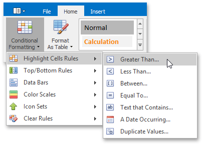
•On the Home tab, in the Styles group, select Conditional Formatting | Highlight Cells Rules, and then select one of the following items: Greater Than..., Less Than..., Between... or Equal To...
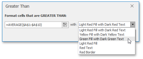
•In the invoked dialog, specify the threshold value, and select formatting options to be applied to cells that meet the condition. Note that you can also use a formula to specify the threshold value. If you enter a formula, start it with an equal sign (=). If a formula returns an error, formatting options will not be applied.
Format Cells that Contain Text or a Date
To highlight cells that contain the specified text string or time period, do the following:
•Select the cell range to which you wish to apply a conditional format.
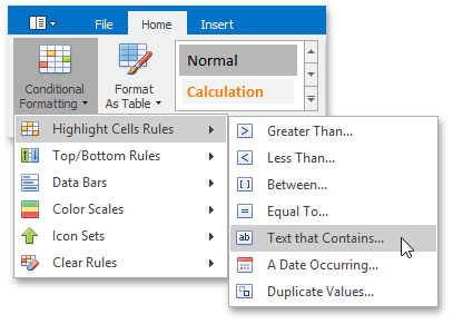
•On the Home tab, in the Styles group, select Conditional Formatting | Highlight Cells Rules, and then click Text that Contains... or A Date Occurring....
•In the invoked dialog, specify the text string (if you selected Text that Contains...) or time period (if you selected A Date Occurring...) to be highlighted, and select the formatting options to be applied to cells that meet the condition.
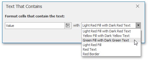
Note that for the Text that Contains... rule you can also specify a formula that returns text. If you enter a formula, start it with an equal sign (=). If a formula returns an error, formatting options will not be applied.
Format Unique or Duplicate Cells
To find unique or duplicate values in a range of cells, do the following:
•Select the cell range to which you wish to apply a conditional format.
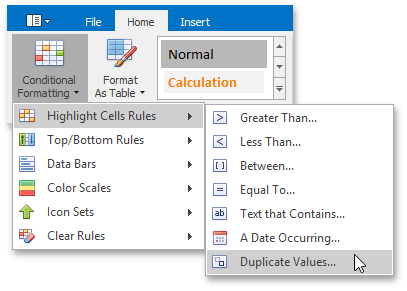
•On the Home tab, in the Styles group, select Conditional Formatting | Highlight Cells Rules | Duplicate Values...
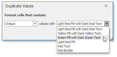
•In the invoked dialog, specify whether you wish to highlight unique or duplicate values, and select the formatting options to be applied to cells that meet the condition.
Format Top or Bottom Ranked Values
To highlight only the top or bottom ranked values in a range of cells, do the following:
•Select the cell range to which you wish to apply a conditional format.
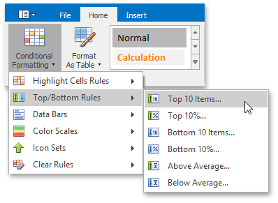
•On the Home tab, in the Styles group, select Conditional Formatting | Top/Bottom Rules, and then select one of the following items: Top 10 Items..., Top 10%..., Bottom 10 Items... or Bottom 10%...
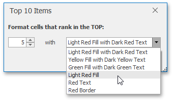
•In the invoked dialog, specify the number or percentage of the rank value (depending on the selected rule), and select the formatting options to be applied to cells that meet the condition.
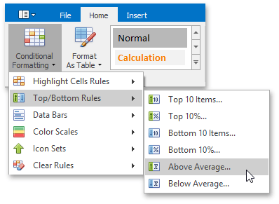
Format the Cells whose Values are Above or Below the Average
To highlight values that are above or below the average in a range of cells, do the following:
•Select the cell range to which you wish to apply a conditional format.
•On the Home tab, in the Styles group, select Conditional Formatting | Top/Bottom Rules, and then click Above Average... or Below Average...
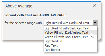
•In the invoked dialog, select the formatting options to be applied to cells that meet the condition.
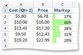
Format Cells using Data Bars
The data bar conditional formatting rule draws a shaded bar in the background of each cell in the range to which the rule is applied. The length of the data bar represents the cell value. A longer bar represents a higher value, and a shorter bar represents a lower value. For example, the image below shows markup magnitude using solid light-green data bars.
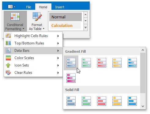
To apply a data bar conditional formatting rule, do the following:
•On the Home tab, in the Styles group, choose Conditional Formatting | Data Bars, and then select the desired color for a gradient or solid data bar.
Format Cells using Color Scales
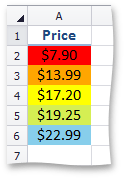
Color scales compare values using a gradation of two or three colors. The shade of the color represents higher, middle and lower values in the cell range to which the rule is applied. For example, the image below shows a price distribution using a gradation of three colors. Red represents the lower values, yellow represents the medium values and sky blue represents the higher values.
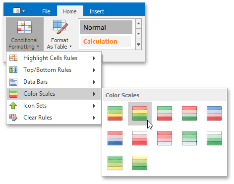
To create a color scale, do the following:
•On the Home tab, in the Styles group, choose Conditional Formatting | Color Scales, and then select one of the predefined color combinations.
Format Cells using Icon Sets
An icon set conditional format classifies data in a range into three to five categories. The Spreadsheet divides the range into equal parts based on the number of icons in the selected set and applies an icon to each cell depending on its value. For example, the image below shows the value ranking. A filled star represents values that are greater than or equal to 67 percent, a half-filled star represents values that are less than 67 percent and greater than or equal to 33 percent, and an empty star shows values that are less than 33 percent.

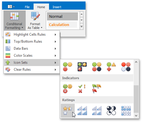
To apply an icon set conditional formatting rule, do the following:
•On the Home tab, in the Styles group, choose Conditional Formatting | Icon Sets, and then select the desired icon set from the gallery.
Clear Conditional Formatting Rules
To delete a conditional formatting rule, do one of the following:
•Select the range that contains the conditional formatting rules you wish to clear. On the Home tab, in the Styles group, select Condtional Formatting | Clear Rules | Clear Rules from Selected Cells to delete the rules applied to the selected range.
•To clear all conditional formatting rules on a worksheet, select Condtional Formatting | Clear Rules | Clear Rules from Entire Sheet.
Copyright (c) 1998-2016 Developer Express Inc. All rights reserved.
Send Feedback on this topic to DevExpress.